My Special Project (Recognition of Hand Written Digits Through PCA)

The Principal Components Analysis (PCA) algorithm has been very useful in many applications such as image compression and decreasing the dimensionality of high-dimensional datasets.  The PCA is a statistical implementation of finding the eigenvectors which represent the dataset.  These eigenvectors are arranged according to the variance of the data in a specific dataset.

Entry 20: Image Compression

In previous times, every bit of storage seems so significant , but because of recent technological developments, storage capacity has been developed to quite large sizes that even a megabyte seems so useless already.

Even though the "phenomenon" of less storage size appreciation and the prices of storage media are decreasing, compression techniques to minimize the storage size of files are still being used and developed.

In this activity, we come to realize a basic method of compressing an image file through the discrimination of some of the image's details without so much information loss brought to the compressed image.

The method used in this activity is called PCA or the Principal Components Analysis.  It is based on the concept of identifying the eigenvectors of the image with the highest information contribution based on the eigenvalue of the diagonalized covariance matrix of the  n-dimensional "observations".  This results to a minimized number of information stored in the resulting compressed image, thus, the image size is smaller than the original.

For this activity, I chose the image in Fig. 1 to be my test image to be compressed.

Figure 1:  Original image to be compressed.

We first sampled the image such that size of each subimage is 10x10.  From the ensemble of these subimages, we computed the PCA using the pca() function in scilab.

One of the results after computing the PCA is the eigenvectors of the image.  The eigenvector of the image used here is shown in Fig. 2,

Figure 2:  Eigenvectors for the image.

After the eigenvectors were computed, we identified the eigenvectors with high explained variance to be used on the compression.  In the plot below (Fig. 3), we can see the variance explained by each eigenvectors.

Figure 3:  Scree plot.  Blue) Percent of variance explained by each eigenvector; Red) Cumulative sum of the variance explained of the eigenvectors.

We utilized different number of eigenvectors to achieve certain compression levels.  Some compressed images at different compression levels are shown in Fig. 4,

Figure 4:  Samples of compressed images using PCA. (from top to bottom) 92%, 95%, 97%, 99% and 100% compressed images.  The number of eigenimages required to compress the image to these compression levels are (from top to bottom) 1, 2, 4, 13 and 100 eigenimages, respectively.

For the compression, the number of stored information is decreased depending on the number of eigenimages utilized.  It is nice to know that the highest eigenvector explains almost 92% of the entire image.  This implies that even if small number of eigenimages were used in the reconstruction, the quality of the result will not deteriorate much.

In this activity I would rate myself 10/10.

Source:
    Activity Sheet for Activity 14 - Dr. Maricor Soriano

Entry 19: Color Image Segmentation

Images contain many information that can be retrieved through image processing.  Some of the information can be used to discriminate certain regions (regions of interest - ROI) as the important regions and put other regions not containing the specified region to a null value forcing other points to be a part of the background.

In this activity, we perform the method of color image segmentation to identify in the entire image the regions with the same information with the reference patch.  For this to be done, normalization of the color channels was performed given by the equation below.

 

We studied the two types of color image segmentation techniques, the parametric and the non-parametric color segmentation.  The parametric segmentation method utilizes the Gaussian distribution wherein the probability of the image value depends on the reference patch.  The mean of each color channel was used to be the abscissa with the highest probability.  The Gaussian distribution used in the parametric technique is stated below,

 

the spread and mean parameters of the distribution comes from the standard deviation and the mean value of the reference patch, respectively.

We used the technique of color image segmentation to the image below (My Toy Car :D) shown in Fig. 1,

Figure 1:  Image to be segmented

It is important to realize that we utilizes the Normalized Chromaticity Space in representing the location of the values to be calculated from the patch.  Also, this chromaticity space will help us visualize quantitatively what colors are present in the image.  A sample normalized chromaticity graph is shown below in Fig. 2,

Figure 2:  Sample Normalized Chromaticity Space

To continue with the parametric image segmentation, we chose a patch in the ROI to represent the entire region.  The patch chosen appear to have a large color component of yellow Fig. 3.

Figure 3:  Reference color patch for color image segmentation.

After doing the algorithm of taking the Gaussian probabilities and multiplying the results with each other, we get a parametrically segmented version of Fig. 1 as shown in Fig. 4.

Figure 4:  Segmented image through parametric color image segmentation.

Our next task is to segment the original image using the non-parametric approach.  In this technique, it requires the knowledge of the histogram of the normalized chromaticity space for the entire image and the patch representing the ROI.

For the image to be segmented, we calculated the 2D normalized chromaticity space histogram representing the entire image.  The computed histogram is shown in Fig. 4 along with the normalized chromaticity space representing the entire color spectrum.

Figure 4:  Left) The normalized chromaticity histogram representing the image, Right) the normalized chromaticty space fot the entire color spectrum.

We also computed the normalized chromaticity histogram for the patch chosen to represent the ROI.  In Fig. 5, we superimposed the computed normalized chromaticity histogram of the ROI to the normalized chromaticity space representing the entire color spectrum to properly visualize the color component representing the ROI.

Figure 5:  Superimposed normalized chromaticity histogram of the chosen representative region for the ROI with the normalized chromaticity space of the entire color spectrum.

It can be observed in Fig. 5 that the representative color of the ROI is near the yellow-orange region of the normalized chromaticity space of the entire spectrum.

We performed histogram backprojection which will yield the non-paramtrically segmented image.  The resulting non-parametrically segmented image is shown in Fig. 6.

Figure 6:  Resulting non-parametrically segmented image.

It is so handy to the techniques performed above to identify regions of interest.  Many applications of these methods can be made such as tracing the trajectory of certain material.

In this activity I want to give myself a 10/10 because of my efforts and enthusiasm in doing the activity.  I learned much in this activity which is  the most important thing for me.

Source:

    Activity Sheet for Activity 13 - Dr. Maricor Soriano

Entry 18: Color Camera Processing

Before this I took this course I was so naive about some things and included in those things is the concept of white balance.

I hear the term before but I never even bother to take some time to Google any information about it.  But after performing this activity, I truly appreciated the white balancing algorithms as they transform images taken with different light sources to maintain their color signatures.

In this activity, we explored two common method being utilized in white balancing namely, White Patch Algorithm and the Gray World Algorithm.

We first take images of a single scene with a white material in it using different white balancing modes in a digital camera. 

Given these images, we sampled an image with the least appropriate white balance setting for the lighting condition during the image was taken. From this data, we can start implementing the two algorithms mentioned above.

First, we implemented the White Patch Algorithm.  A requirement of the White Patch Algorithm is that a white patch must be present in the image to be a reference or the normalizing value.  Thus, we chose from the image a pixel with white value and inputted it to the algorithm.  Shown in Fig. 1 is the image captured under a sunlight lighting with a white balance mode of "Incandescent" set in the digital camera.

Figure 1:  Image with inappropriate white balance setting (Incandescent) used in the lighting condition (Sunlight).

The White Patch Algorithm simply normalizes the entire image with the chosen white patch from the image itself.  After the normalization, we formed the image array and reconstructed the image.  The result is shown in Fig. 2 - White Patch Algorithm applied to the original image (Fig. 1).

Figure 2:  Resulting image after the White Patch Algorithm has been applied to the original image.

It is quite noticeable that a significant change in the image can be observed.  The white bond paper lost the "bluish stain" after the algorithm was applied and it appears to be very pure white.  The other colors can be seen to have improved and look more like in the real world.

The next algorithm that will be performed is the Gray World Algorithm.  In this method, the mean of each color channel is the variable used to normalize each of the values in the respective channels.  We performed this technique to the original image and the result is shown in Fig. 3,

Figure 3:  Resulting image after the Gray World algorithm was applied to the original image.

In Fig. 3, the resulting image appear to be have a higher intensity but the white bond paper looks so pure white.  On the other hand, the other colored objects seem to be flooded by the white contrast.

The next aspect we looked at is the accuracy and efficiency of the two algorithms.  To do this, we took an image of collection of object sharing the same shade of hue with no white in the background.  The image used is shown in Fig. 4,

Figure 4:  Image with inappropriate white balance (Incandescent) with objects sharing the same shade of hue under a fluorescent lighting.

We performed both algorithms in this image and the results are shown in Fig. 5,

Figure 5:  Left) White Patch Algorithm, Right) Gray World Algorithm applied to the original image.

We have observed that the White Patch Algorithm is better used when the colors in the spectrum is not well represented in the image.  Even though the image appeared grainy after the application of the White Patch Algorithm it still appeared more crisp relative to the result after the gray World Algorithm has been applied to the images.

The possible reason why the White Patch Algorithm is suited in the case when only a small portion of the color spectrum is represented in the image is that for the Gray World Algorithm, the mean of the entire color channel is being used in the normalization, thus, since other colors are not represented the result of the normalization will probably not give the true white balance for the image.

In the succeeding figure, the results of  the implementation of both algorithms are shown for various white balance setting used in capturing the scene.  In the first column of the figures below show the images after the White Patch Algorithm has been implemented to the original images which are those in the middle column, while the last column corresponds to the result after the Gray World Algorithm has been applied.

Figure 6:  Left) White Patch Algorithm applied to the original image; Middle) Original image under "Cloudy" white balance mode; Right) Gray World Algorithm applied to the original image.

Figure 7:  Left) White Patch Algorithm applied to the original image; Middle) Original image under "Fluorescent 1  " white balance mode; Right) Gray World Algorithm applied to the original image.

Figure 8:  Left) White Patch Algorithm applied to the original image; Middle) Original image under "Fluorescent 2" white balance mode; Right) Gray World Algorithm applied to the original image.

Figure 9:  Left) White Patch Algorithm applied to the original image; Middle) Original image under "Fluorescent 3" white balance mode; Right) Gray World Algorithm applied to the original image.

Figure 10:  Left) White Patch Algorithm applied to the original image; Middle) Original image under "Incandescent" white balance mode; Right) Gray World Algorithm applied to the original image.

In this activity I would give myself a 10/10 for the completeness of the result despite of late posting.

Source:
     Activity Sheet for Activity 12  - Dr. Maricor Soriano

Entry 17: Playing Notes by Image Processing

When I was in elementary, I started to learn the basics of Music Theory.  I learned to read notes and other musical symbols.  I practiced how to play the piano.  I was really happy when I was able to hear the music coming from the piano.

Another happy music moment was when I started to study playing the violin.  I learned to play the violin in tutorials available in the Internet.  By then, I started saving money to buy my own violin.

This time around, again I felt a happy music moment when I knew that this activity will be about playing musical pieces through image processing. 

The goal of this activity was to "read" notes and "play" them using all of the methods learned in the previous activities.

To perform this, we first chose a simple musical piece - Twinkle Twinkle Little Star.  Next, to further simplify the process, we cropped the staffs from the musical piece (Fig. 1).

Figure 1:  Sample cropped staff from the music sheet.

With the staff in hand, we performed custom methods to classify the notes in the staff.  The critical information in this piece of image are the pitch of each note and the length of each note playing time.  Rests are not present in this piece so our task was a lot easier.

We cleaned the staff image and introduced morphological operations (successive erosion and closing).  The goal of this task is to characterize the notes on the piece and get their individual pitch and playing time information.

Figure 2:  Sample cleaned staff using erosion and closing.

We took the coordinates of the center of mass of each blob and compared it against the "known" coordinates of the staff's ledger lines.  This information will give us the pitch of the note.  Also, the area of the blobs representing the notes were taken to determine the type of note (i.e. quarter or half note).  Notice that half notes have a smaller area than the quarter note, thus, we can differentiate one from the other.

After the gathering of all the informations in the sheet, we inputed them in the function wavwrite() which converts an array of sinusoids with frequencies corresponding to each musical notes to a .wav music file.

After all of the procedures, finally the piece was already converted into a musical format and we were able to play it in our computer!  I used PiTiVi Video Editor in Ubuntu to render the video.

In this activity I would give myself a grade of 10/10 because of my efforts in finishing this activity.  Also, I have found an easy way of reading the piece without using imcorrcoef().

Source:
    Activity Sheet for Activity 11 - Dr. Maricor Soriano

Entry 16: Binary Operations

Ola!  In this activity, we performed binary operations to identify simulated normal cells and discriminate cancer cells from normal cells.  We implemented our knowledge of morphological operations to achieve our goal.

We performed the method of classifying the normal cell area by first taking patches of 256x256 pixels from the original image.  This process was implemented by randomly taking a point from the original image and acquire the patch starting at that point, this way, the bias was reduced.  Samples from the randomly chosen patches are shown in Fig. 1 along with the binarized version with the threshold equal 0.84.

Figure 1: Sample of the 256x256 patches from the original image and their corresponding binarized versions.

The binarized version was done by choosing a threshold based from the pixel value histogram as shown in Fig. 2,

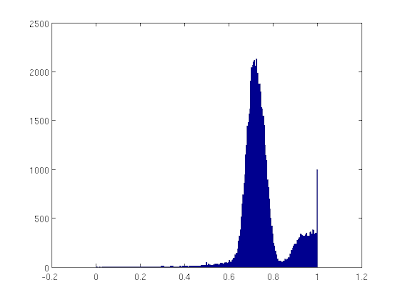Figure 2:  Pixel value histogram of a sample patch indicating that the threshold is near the value of 0.85.

After generating the binarized patches, we identified the distribution of area of contiguous regions using the function bwlabel().  The histogram of the contiguous regions from the entire subimages are shown in Fig. 3.  It must be noted that we limited the reasonable area to be counted in the histogram in the range 50px to 1000px only.  Values outside the specified range are assigned to be outliers.

Figure 3:  Histogram of the area of contiguous regions in the patches.

In Fig. 3, we observed that the most probable area is about 500px.  Thus we conclude that a normal cell has a mean area of 500px.

Now, we find a method to identify a cancer cell in a region with normal cells.  We utilized the computed area of a normal cell and used it in the discrimination method.  We know that when a region of smaller area is applied with the open morphological operation with a structuring element with a larger area, the region will vanish.  Since the the cancer cells are relatively larger, it is possible to remove the normal cells by opening the image with the structuring element with area equal to the normal cell.

After applying the method, we have successfully determined the cancer cells from the rest of the normal cells as shown in Fig. 4.

Figure 5:  Image of normal cells with randomly located cancer cells.  Also shown are the detected cancer cells.

Based from the results, we have verified the application of binary operations in identifying cancer cells in an ensemble of normal cells.

In this activity I developed a better grasp of the concept of morphological operations and I learned that extensive applications may be adapted using the basic morphological operations in binarized images.  I'll be rating myself 10/10 because I completed all the requirements for this activity and also because of the knowledge I gained.

Source:
    Activity Sheet for Activity 10 - Dr. Maricor Soriano
    Thanks to BA Racoma for giving me a tip regarding the open operation. :D

Entry 15: Morphological Operations

Morphological operations are methods in transforming an image by using a specific structuring element to yield desired formation in the image.  This technique is widely used in image processing to produce a more easy-to-handle image.

Two main morphological operations are used in this activity which are the dilate and the erode operations.

The erode operation is defined mathematically as,

this means that every points in B must be contained in A so that the value in A where the origin of B is located will attain a value, else, a zero value will be assigned to that B location.

Graphically it can be illustrated by the image below.

The dilate operation on the other hand is defined mathematically as,

the implication of this equation is that when B covers a location in the background, provided that the origin of B is contained in A, then the background region covered by B will take the value of the foreground.

An illustration is shown by the image below.

Below (Fig. 1) are the images to be structured and (Fig. 2) are the structuring elements used.

Figure 1:  Images to be structured.

Figure 2:  Structuring elements used in the process.

In the succeeding images, we show the results of dilating the original images (Fig. 1) with the strels (Fig. 2).

Figure 3:  Dilated images using a 1x2 strel.

Figure 4:  Dilated images using a decreasing diagonal strel.

Figure 5:  Dilated images using a 2x1 strel.

Figure 6:  Dilated images using an increasing diagonal strel.

Figure 7:  Dilated images using a 2x2 strel.

Figure 8:  Dilated images using a cross strel.

After determining the dilated images, we tried another morphological operation which is erosion.  The images below are the eroded original (Fig. 1) images using the strels in Fig. 2.

Figure 9:  Eroded images using a 1x2 strel.

Figure 10:  Eroded images using a decreasing diagonal strel.

Figure 11:  Eroded images using a 2x1 strel.

Figure 12:  Eroded images using an increasing diagonal strel.

Figure 13:  Eroded images using a 2x2 strel.

Figure 14:  Eroded images using a cross strel.

Morphological operations can be applied to different image processing problems to simplify them.  The usefulness of these operations depend on the user.

In this activity I would rate myself a grade of 10/10.

Source:
    Activity Sheet for Activity 9 - Dr. Maricor Soriano

Entry 14: Enhancement in the Frequency Domain

Speaker: Fourier transform enables us to travel across dimensions!  

Audience: How?!!!

Speaker: It's because Fourier transform empowers us to see the world of the inverse dimensions!

Audience: Ok...


This activity emphasizes the power of Fourier Transform (FT) in various applications.  To be discussed here are the simple exercises made to get a better idea on how FT changes some properties of our object.  Also, a major application of FT will be included here which is about using FT in cleaning digital finger print images.  The application of FT in filtering repetitive patterns of "noise" in painting due to its canvas weave and removal of vertical lines in a photograph was used to correct these issues and to produce a better image.

So we first simulated the action of FT on basic patterns as shown in the FT pairs below (Fig. 1).

FIgure 1:  Fourier Transform pair of different basic patterns (symmetric dots, symmetric circles and symmetric squares).

Also the FT pair of the Gaussian pattern was simulated.

In the next section, we performed enhancement of a fingerprint image using filtering techniques in the Fourier space of the image.  The image of the fingerprint is shown in Fig. 2,

Figure 2:  Original image of the fingerprint to be "cleaned".

To start filtering, we first identify how the frequency world of the fingerprint image look like so that we can identify the proper filtering mask to use to discriminate unwanted information in the image.

In Fig. 3, the FT of the fingerprint image is shown which reveals the nature of the frequency of the information in the image.

Figure 3:  Fourier Transform of the fingerprint image which shows the frequency component of the image.

We realize based from the information from Fig. 3 that the frequency of the information relevant to the fingerprint is not well distinguishable from the noise so we chose a smoothing mask to use to smoothen the noise in the image and from that smoothened image, we can do thresholding to determine the actual fingerprint image discriminating the noise.

We show in Fig. 4 the mask used to filter the fingerprint image.  The mask is composed of two Gaussian functions, one with a very small variance to facilitate the filtering of the DC component and the other Gaussian filter is responsible to discriminating the noise of high frequencies.

Figure 4:  Double Gaussian filter to clean the fingerprint image.  Sigma used are 0.0001 and 18 to filter the DC and high frequency components of the noise.

After applying the filter to the original fingerprint image, we now have the smoothened/filtered version.  The result is shown in Fig. 5.

Figure 5:  Left) Filtered image using the double Gaussian filter, Right) Thresholded filtered image showing the significant details of the fingerprint showing that the noise were wiped out.

Also shown in Fig. 5 is the final filtered image of the fingerprint.  After taking the smoothened image, we applied thresholding to it to wipe away any traces of noise in the background to only leave the significant components constituting the fingerprint.

The next task is to remove vertical artifacts from one of the images of the moon's surface (Fig. 6).  It was said in the image details that the artifact was due to the concatenation of individual framelets to make the entire image [1].

Figure 6:  Original image of the moon's surface with evident vertical lines.

To start the process of filtering the vertical lines in the image, we first converted the image into a grayscale version and took the FT of it to reveal the frequency values in the image (Fig. 7 - Left).

Figure 7:  Left) Fourier Transform of the grayscaled moon image showing repetitive dots along the x-axis, Right) Filtering mask used to remove the vertical lines.

From our Activity 7, we learned that the FT of vertical lines correspond to a series of dots in the x-axis of the frequency space.  Thus we made a filtering object that masks the points where the information relating to the vertical lines were located (Fig. 7 - Right).

After applying the mask to the image's FT and going back to the linear domain, we produce the filtered form of the image.  In Fig. 8, shown are the original image along with the filtered image of the moon.

Figure 8:  Left) Original grayscale image of the moon with evident vertical lines, Right) Filtered image wherein the vertical lines were removed.

Lastly, we performed the same method to a painting.  The task is to remove the effect of the canvas weave on the image.  The original image is shown in Fig. 9.

Figure 9:  Original image of the painting with very obvious canvas weave pattern.

We get the grascale of the image of the painting and took the FT of it to reveal the localized high valued frequencies.  Localized high valued frequencies can be thought to carry the information of the frequently occurring canvass weave pattern and there we based the mask to be used for filtering.  The FT of the image and the mask is shown in Fig. 10.

Figure 10:  Left) FT of the painting image showing localized high valued frequency, Right) Mask developed to filter the canvass weave pattern.

After applying the mask to the FT of the image and returning back to the linear domain, we get the filtered image wherein the canvass weave pattern can no longer be seen.  In Fig. 11, shown side by side are the original grayscaled image of the painting along with the filtered image.

Figure 11:  Left) Original grayscaled image of the painting, Right) Filtered painting showing no signs of the canvass weave pattern.

The last thing we did in this activity is to show the image of the mask used in linear domain.  We can see in Fig. 12 the similarity of the linear domain version of the mask used to the canvass weave pattern.

Figure 12:  Linear domain version of the mask used in the filtering of the painting.

In this activity I would give myself a 10/10 for the dedication and the learning I had during this activity.

Source:

    [1]  Activity Sheet for Activity 8 - Dr. Maricor Soriano